Data Modeling Fundamentals part-2: Data Modeling Approach and Techniques

Welcome readers of data engineering blog, after taking a break on January finally I release the second part of data modeling. Last year, in https://datarunner01.hashnode.dev/data-modeling-fundamentals-part-1-introduction-to-data-model-and-data-modeling-types , I already write about what is data modeling, data modeling type, etc. This time, I want to go deeper into data modeling approach to support business process.

Choosing the right data modeling approach serves as the foundation for reliable business intelligence. We’ll break down the core data modeling approach with practical examples and implementation.

Data Modeling Approaches for OLTP

Databases are made for OLTP and are optimized to effectively manage large numbers of real-time transactions. Ensuring data integrity, reducing redundancy, and optimizing for frequent read/write operations (CRUD) are the primary objectives. To manage these actions without compromising data integrity, the database must guarantee ACID (Atomicity, Consistency, Isolation, Durability) compliance.

In the context of database design, normalization is a technique that arranges tables to minimize insertion, deletion, and update anomalies by removing redundant data, hence reducing redundancy and dependency of data. Denormalization, on the other hand, is the opposite of normalization in which redundancy is purposefully added to the data to enhance data integrity and performance for the particular application. These two database modeling strategies will be explained in the next section.

Normalization

Normalization is the process of changing a database to improve data consistency and integrity while decreasing redundancy. Using this method, a data model is divided into several connected tables, each of which holds a distinct set of data. The objective is to minimize anomalies and preserve data integrity.

Let’s explore the different types of normalization with examples:

• First Normal Form (1NF)

The first step in the database normalization process is called First Normal Form (1NF). 1NF Form guarantees that every table column has only atomic values, which means that no repeating data groupings. Imagine an early-stage e-commerce application storing order data like this:

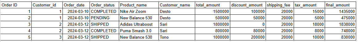
E-commerce database schema: order table | Image create by author

What make this 1NF?

➡️ A single product that a consumer has bought is now represented by each row
➡️ There are atomic values (no lists or sets) in every column

• Second Normal Form (2NF)

Second Normal Form (2NF) requires that each non-key column is fully dependent on the primary key, which means it cannot contain any partial dependencies. In 2NF, all of the non-key columns must rely on the entire main key, not just a certain portion of it. Imagine an early-stage e-commerce application storing order data like this:

(a) order table

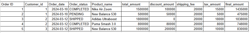
E-commerce database schema: order table | Image create by author

(b) customer table

E-commerce database schema: customer table | Image create by author

(c) product table

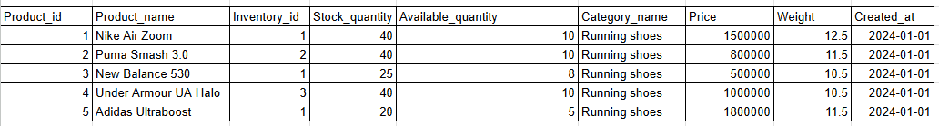
E-commerce database schema: product table | Image create by author

What make this 2NF?

➡️ Every non-key column depends on the entire primary key

➡️ Separate inventory data on product table into new customer table

• Third Normal Form (3NF)

Third Normal Form (3NF) is a classical relational database modelling approach that minimize data redundancy by requiring that each non-key column rely solely on the table's primary key. The next step after attaining 2NF is to make sure that there are no more transitory dependencies. Imagine an early-stage e-commerce application storing order data like this:

(a) order table

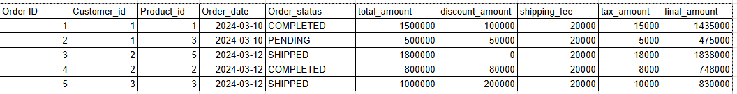
E-commerce database schema: order table | Image create by author

(b) customer table

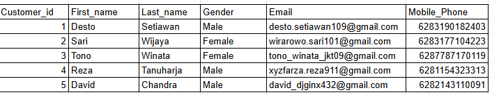
E-commerce database schema: customer table | Image create by author

(c) product table

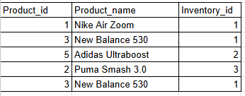
E-commerce database schema: product table | Image create by author

(d) inventory table

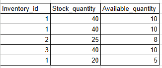
E-commerce database schema: inventory table | Image create by author

What make this 3NF?

➡️ There are no partial dependencies on a composite primary key

➡️ All non-key attributes must depend directly on the primary key, and nothing else.

➡️ Separate customer data on order table and inventory data on product table into new customer table and inventory table

• Boyce-Codd Normal Form (BCNF)

The 3.5 NF is another name for the Boyce Codd Normal Form. Higher than 3NF, this degree of normalization is frequently applied in OLTP to remove redundancies and update abnormalities. It guarantees that the left side must be a superkey for each functional dependency.

Imagine an early-stage e-commerce application storing order data like this:

(a) product table

E-commerce database schema: product table | Image create by author

(b) product variant table

E-commerce database schema: product variant table | Image create by author

(c) variant table

E-commerce database schema: variant table | Image create by author

• Fourth Normal Form (4NF) and Fifth Normal Form (5NF)

Fourth Normal Form (4NF) and Fifth Normal Form (5NF) addresses a situation which one entity has several independent relationships. Although they exist, 4NF and 5NF are not frequently used. In simpler systems, 4NF and 5NF are rarely needed, but it becomes important in more complex OLTP schemas.

Denormalization

Denormalization is a form of data modeling similar to a normalized model, but with less emphasis on normalization principles. This method is distinguished by the storage of redundant data across several tables which is frequently employed when performance is a primary concern. It reduces the need for numerous joins and simplifies complicated queries.

When to Choose Normalization or Denormalization?

The tables below summarize the trade-offs between normalization and denormalization:

Comparison Table: Normalization vs Denormalization | Image create by author

Data Modeling Approaches for OLAP | Analytics Data Modeling

Analytics data modeling for Online Analytical Processing (OLAP) is the process of structuring large volumes of historical data to enable rapid, multi-dimensional analysis. Data should be arranged according to the chosen model type so that it is easy to understand where it is stored and optimized for read-heavy workloads like business intelligence (BI) and reporting.

There are some type of key used for primary key in analytics modelling, which prevents duplication and ensures data integrity.

• Natural key

Primary key that is directly from the data source system unique identifier and inherent business meaning. They are derived from real-world attributes and may include values.

• Surrogate key

Primary key that is a system-generated unique identifier with no business meaning to identify a record in a table. Surrogate keys offer a single-column primary key for every table, which makes data warehouse to improve query performance, simplify joins, and enable effective data tracking.

• Composite key

A primary key can consist of two or more columns to ensure uniqueness at a granular level. Composite keys are derived from real-world values and carry meaningful information.

There are 4 analytics data modeling strategies will be explained in the next section.

Dimensional modeling

Dimensional modeling is primarily used in data warehouse and business intelligence environments. Dimensional modelling is best suited for decision support, reporting, and analytical querying. In dimensional modeling, the most popular approach to designing a data warehouse is using a star schema, snowflake schema, or galaxy schema.

Dimensional modeling includes facts and dimensions.

• Dimension table

Each dimension table contains flat denormalized attribute data that includes numerous low-cardinality texts that describe the business activity. Dimension tables provide context for the information kept in fact tables. This dimension table use 5 W’s and 1 H to helps users understand the context surrounding a business process.

There are different types of dimension tables:

(a) Conformed dimension: this dimension table shared across multiple fact tables in a single database, or across multiple data marts or data warehouses.

Example: A time dimension used across sales, inventory, and customer tables.

(b) Slowly Changing Dimension (SCD): this dimension table need to manage changes data over time in the data warehouse.

Example: A customer dimension storing address history.

Before implement any slowly changing dimensions, the next question to ask is if the business needs to store the history or not? What your company can truly measure depends on how you model these changes. Slowly Changing Dimension tables come in a variety of popular forms.

➡️ SCD type 1: Overwrite Old Values

This method is used when data can change, but you don’t need to keep the old values. Every time something changes, the new value replaces the previous one.

➡️ SCD type 2: Track History with new Rows

This method is by creating multiple records for a given same natural key in the dimensional tables with separate surrogate key and metadata like timestamps or flags to different version numbers. A complete history of changes is maintained by inserting a new row for every version rather than overwriting the previous value.

➡️ SCD type 3: Track Limited History with new Attribute

This method track changes in a row by adding a new column for the previous value. The Type 3 preserves limited history as it is limited to the number of columns designated for storing the last_<insert_name> and current_<insert_name>.

(c) Junk dimension

Junk dimension is a single table with a combination of different and unrelated attributes for better data organization. Junk dimensions are often created to manage the foreign keys created by changing dimension to preserve historical data.

Example: A marketing survey junk dimension containing attributes such as “opted for email” and “attended the webinar.”

(d) Degenerate dimension

A degenerate dimension is a dimension key that does not require a separate dimension because it is located directly in the fact table.
These are basically dimension keys with no further properties.

Example: A transaction ID in a sales fact table.

• Fact table

A fact table is the central component of a dimensional model that represents business events or transactions. It keeps track of quantifiable measures that hold information about a company's business performance like sales income, amount sold, or website clicks. Facts are almost always have numeric value.

There are different types of fact table:

(a) Transaction Fact Tables

Transactional facts capture individual business events or transactions at the most atomic level of a business process. These tables are very helpful for examining sales trends, customer behavior, and operational effectiveness.

Use Cases: sales invoices, bank withdrawals, or website clicks

(b) Periodic Snapshot Fact Tables

Periodic snapshot fact capture aggregated data to provide a summarized view of metrics over regular time intervals. It might be a snapshot of what happened over the course of a week or a month.

Use Cases: End-of-month inventory, daily bank balances, or monthly account activity

(c) Accumulating Snapshot Fact Tables

Accumulating snapshot fact tables are designed to track the stages of a business process or workflow. Stakeholders can track progress and spot bottlenecks by gathering snapshot facts, which offer insights into the lifecycle of projects or processes.

Use case: An order fulfillment fact table indicating stages such as "shipped" and "delivered"

(d) Factless Fact Tables

Factless fact tables is a special type of table that captures relationships and events without containing any numerical or measurable facts. Factless facts contains only foreign keys to provide context that enabling stakeholders to derive insights.

Use case: A marketing campaign fact table tracking customer attendance at events

Comparison Table: Fact Table Type | Image create by author

I. Dimensional modeling methodologies

☑️ Kimball methodology

The Kimball method initiated by Ralph Kimball is considered to be a bottom-up design approach. When designing the data warehouse, this approach is frequently referred to as dimensional modeling. This approach facilitates quick data analysis and querying to address certain queries about business procedures or subject areas.

Three common data modelling on Kimball method:

(a) Star Schema

A star schema is a dimensional modelling technique used in databases and data warehouses to organize data for easy analysis and understanding. The structure of the star schema is kept straightforward using denormalized structure dimension tables. Although there may be some redundancy in the dimension tables, the star structure helps to enhance query efficiency by lowering the number of joins needed.

Key Characteristic

➡️ There is just one main fact table that contains quantitative metrics

➡️ The dimension tables of a star scheme are not directly related to one another

➡️ Star schemas are intended for quick, read-heavy analytical

➡️ Star schemas are easier to use with BI tools and work well with datamarts

Snowflake Schema Example Made from Dbdiagram.io | Image create by author

(b) Snowflake Schema

Snowflake schema is an extension of the star schema that further normalizes dimension tables, resulting in a more normalized structure. In the snowflake schema, dimension tables are further divided into related tables or sub-dimensions, which has a more standardized structure. It can be beneficial for specific query patterns and allows for more effective storage.

Key Characteristic

➡️ There is just a single primary fact table that contains quantitative metrics, some of which have been standardized into additional sub-dimensions

➡️ The dimension tables of a snowflake schema can be connected to one another

➡️ Snowflake schema attributes are only stored once in normalized tables, making data updates and maintenance easier

➡️ Query performance may be slowed down by the need for more complex SQL queries with multiple joins when querying data

Snowflake Schema Example Made from Dbdiagram.io | Image create by author

(c) Galaxy Schema

Galaxy schema (also known as a fact constellation) is a collection of several star schemas with shared dimensions that allow for cross-functional analysis. In the snowflake schema, Normalizing data can cut down on redundancy and boost storage effectiveness. In many medium to large businesses, when the demand for several fact tables, this architecture provides enterprise-grade flexibility.

Key Characteristic

➡️ The Galaxy schema reduces data redundancy by having two or more primary fact tables that reflect different business processes

➡️ Fact tables inside galaxy schema share common dimension tables ensuring consistency and enabling cross-functional analysis

➡️ Galaxy schema categorize as complex schema, as it combines elements of multiple star/snowflake schemas

➡️ This schema ideal for large, enterprise-wide data warehouses that need to integrate.

II. Dimensional Modelling Design Process

In the dimensional modelling approach, four key steps guide the design process:

Step 1: Select the business process

Choose the precise event or business activity that needs to be examined, such as inventories, sales, or orders.

Step 2: Declare the grain

Specify the level of detail that the fact table will display, such as daily summaries or individual transactions. This step determines the level of detail associated with measurements from the fact table.

Step 3: Identify the dimensions

Identify the descriptive characteristics (e.g. product, time, customer) that give the information context to fact table later. In order to minimize the amount of joins needed for querying, data from several linked tables in the original model will be combined during this step.

Step 4: Identify the facts

Select the numerical metrics that will be measured and examined, such as quantity and sales amount.
The outcome of this transformation process is a subject-oriented, denormalized data structure that is ideal for analytical querying and data warehousing.

☑️ Inmon methodology

The Inmon method initiated by Bill Inmon is considered to be a top-down design approach. With a particular focus on creating a standardized enterprise data warehouse (EDW), he is known as the "Father of Data Warehousing". This method potentially more time-consuming to integrate all the data models that support all of the organization's data.

Benefit of dimensional modeling:

➡️ Optimized for fast data retrieval and complex analytical queries by minimizing the number of joins needed

➡️ Simplifies the data structure into business-centric concepts, making it more intuitive for non-technical users to query and understand

➡️ Supports techniques like Slowly Changing Dimensions (SCD) to accurately preserve and analyze data changes over time

Cost of dimensional modeling:

➡️ Implementing and managing SCDs or complex ETL pipelines can be time-consuming

➡️ Often involves denormalization, which leads to duplicating data and higher storage requirements

➡️ The transformation process (ETL) required to build these models can introduce delays, making them less suitable for real-time transactional processing

Data vault modeling

Dan Linstedt developed the Data Vault Modeling (v1.0), an agile data modeling methodology and architecture intended especially for building scalable enterprise data warehouses. The Data Vault method provides scalability, flexibility, and the capacity to monitor past data, carry out audits, and trace data history. In Data Vault 1.0, sequence surrogate keys were used to identify a business entity and that had to include dependencies during the loading process as a consequence.

Later on, it developed into a more complex Data Vault version "2.0". Data Vault Modeling (v2.0) is a business intelligence solution that incorporates best practices for modeling, methodology, architecture, and implementation. In Data Vault 2.0, it introduces the concept of hash keys generated by hashing algorithm (like MD5 or SHA-256) to the business key that represent the main business entities.

Data vault’s uses a three-layer architecture consists of three main components:

• Hubs

The business keys of the business objects with the same semantic granularity are stored in a hub entity. A fundamental business concept, such as customer, product, or order, is represented by each hub.

• Links

Links represent the relationship between Hub entities, enabling complex many-to-many relationships without the constraints. A Link table contains the hash keys from its related Hubs, its own hash key, plus the standard metadata fields.

• Satellites

Satellites store the descriptive data or attributes related to hubs or links, like the textual descriptions, timestamps, or numerical values. Since a hub or link may have only one satellite, the hash key of the relevant hub or link is used to identify it.

Benefit of data vault modeling:

➡️ Data vault have modular design allows user to add new data sources or attributes without modify existing pipelines

➡️ It supports massive data volumes (petabyte scale) and high-velocity ingestion through parallel loading

➡️ It inherently stores full historical changes (CDC), allow user to reconstruct the state of data at any point

Cost of data vault modeling:

➡️ The architecture is abstract and requires specialized expertise to design and maintain

➡️ The granular approach and full historical retention significantly increase storage requirements

➡️ Setting up the necessary automation, metadata management, and architecture alignment involves higher upfront effort

Data Vault Schema Example Made from Dbdiagram.io | Image create by author

One Big Table (Wide or Flat tables)

One Big Table (OBT) is a single, massive, flat table that contains both the metrics (facts) and the descriptors (dimensions). Because there are no joins or shuffles, One Big Table (OBT) saves computation, but it requires more storage. In columnar storage systems, where queries can effectively scan just the necessary columns.

Benefit of One Big Table (OBT) modeling:

➡️ By eliminating complex joins, OBT significantly reduces data shuffling, often resulting in query speeds 25–50% faster than traditional star schemas

➡️ Analysts and BI tools can query a single source without needing to understand complex table relationships or write multi-join SQL

➡️ Ingestion pipelines are more straightforward since data moves directly from staging to a flat reporting structure without managing dependencies between multiple tables

Cost of One Big Table (OBT) modeling:

➡️ Storing the same dimensional attributes leads to massive data duplication

➡️ The volume of redundant data in OBT can eventually lead to expensive storage costs as datasets grow

➡️ Adding new data sources or changing existing logic often requires rebuilding the entire table, which can be resource-intensive and prone to synchronization issues

One Big Table (OBT) Schema Example Made from Dbdiagram.io | Image create by author

Anchor Point | Anchor modeling

A data modeling method that enables efficient handling of large volumes of data that changes and historical data over time. The foundation of this approach is a high level normalization (6 NF). Carefully identifying the anchors and their relationships is crucial when using anchor modeling in order to provide a comprehensive and accurate representation of the data.

Benefit of Anchor modeling:

➡️ Changes are made by adding new tables rather than modifying existing ones, keeping old versions functional

➡️ Supports tracking changes over time for both attributes and relationships without disrupting the model

➡️ High normalization reduces data redundancy and duplication

Cost of Anchor modeling:

➡️ Requires a high learning curve and specialized skills

➡️ The high number of joins can lead to significant database load and slower query performance

➡️ Because of the vast number of tables, manual management is unfeasible

Summary

Data modeling is the process of creating a blueprint for database design by defining the structure, relationships, and constraints of data elements. It serves as a single source of truth that simplifies business reporting, prevents confusion over metrics, and ensures data integrity through standardized definitions. Organizations use a progression of conceptual, logical, and physical models to transition from high-level business requirements to technical schemas tailored for specific database systems. This structured approach enhances performance, improves scalability, and reduces storage costs by avoiding redundant or overly complex data structures.

Effective data modeling requires careful consideration of granularity and naming conventions to ensure information remains useful and comprehensible. Advanced techniques like anchor modeling can handle historical data through high normalization, though they often require specialized skills and can impact query performance due to a high number of table joins. Choosing the right database, such as PostgreSQL, provides essential support for transactional integrity and specialized needs like geo-spatial indexing for ride-hailing services. I hope you enjoyed reading this.